AWS Big Data Blog
Use CTAS statements with Amazon Athena to reduce cost and improve performance
Amazon Athena is an interactive query service that makes it more efficient to analyze data in Amazon S3 using standard SQL. Athena is serverless, so there is no infrastructure to manage, and you pay only for the queries that you run. Athena recently released support for creating tables using the results of a SELECT query or CREATE TABLE AS SELECT (CTAS) statement. Analysts can use CTAS statements to create new tables from existing tables on a subset of data, or a subset of columns. They also have options to convert the data into columnar formats, such as Apache Parquet and Apache ORC, and partition it. Athena automatically adds the resultant table and partitions to the AWS Glue Data Catalog, making them immediately available for subsequent queries.
CTAS statements help reduce cost and improve performance by allowing users to run queries on smaller tables constructed from larger tables. This post covers three use cases that demonstrate the benefit of using CTAS to create a new dataset, smaller than the original one, allowing subsequent queries to run faster. Assuming our use case requires repeatedly querying the data, we can now query a smaller and more optimal dataset to get the results faster.
Using Amazon Athena CTAS
The familiar CREATE TABLE statement creates an empty table. In contrast, the CTAS statement creates a new table containing the result of a SELECT query. The new table’s metadata is automatically added to the AWS Glue Data Catalog. The data files are stored in Amazon S3 at the designated location. When creating new tables using CTAS, you can include a WITH statement to define table-specific parameters, such as file format, compression, and partition columns. For more information about the parameters you can use, see Creating a Table from Query Results (CTAS).
Before you begin: Set up CloudTrail for querying with Athena
If you don’t already use Athena to query your AWS CloudTrail data, we recommend you set this up. To do so:
- Open the CloudTrail console.
- On the left side of the console, choose Event History.
- At the top of the window, choose Run advanced queries in Amazon Athena.
- Follow the setup wizard and create your Athena table.
It takes some time for data to collect. If this is your first time, it takes about an hour to get meaningful data. This assumes that there is activity in your AWS account.
This post assumes that your CloudTrail table is named cloudtrail_logs, and that it resides in the default database.
Use Case 1: optimizing for repeated queries by reducing dataset size
As with other AWS services, Athena uses AWS CloudTrail to track its API calls. In this use case, we use CloudTrail to provide an insight into our Athena usage. CloudTrail automatically publishes data in JSON format to S3. We use a CTAS statement to create a table with only 30 days of Athena API events, to remove all of the other API events that we don’t care about. This reduces the table size, which improves subsequent queries.
The following query uses the last 30 days of Athena events. It creates a new table called “athena_30_days” and saves the data files in Parquet format.
Executing this query on the original CloudTrail data takes close to 5 minutes to run, and scans around 14 GB of data. This is because the raw data is in JSON format and not well partitioned. Executing a SELECT * on the newly created table now takes 1.7 seconds and scans 1.14MB of data.
Now you can run multiple queries or build a dashboard on the reduced dataset.
For example, the following query aggregates the total count of each Athena API, grouping results by IAM user, date, and API event name. This query took only 1.8 seconds to complete.
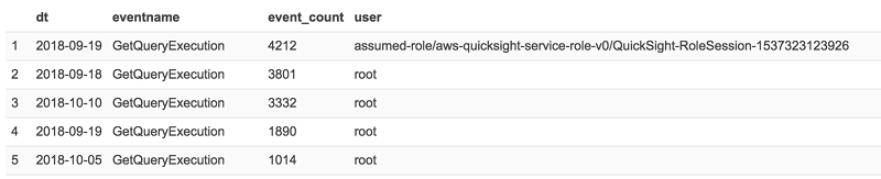
Use case 2: Selecting a smaller number of columns
In this use case, I join the CloudTrail table with the S3 Inventory table while only selecting specific columns relevant to my analysis. I use CTAS to generate a table from the results.
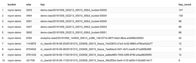
The previous query example returns the last 30 days of S3 GetObject API events that were invoked by the Athena service. It adds the S3 object size and storage class for each event returned from the S3 Inventory table.
We can then, for example, count the number of times each key has been accessed by Athena, ordering the results based on the count from small to large. This provides us an indication of the size of files we’re scanning and how often. Knowing this helps us determine if we should optimize by performing compaction on those keys.
In the case of my example, it looks like this:
Use case 3: Repartitioning an existing table
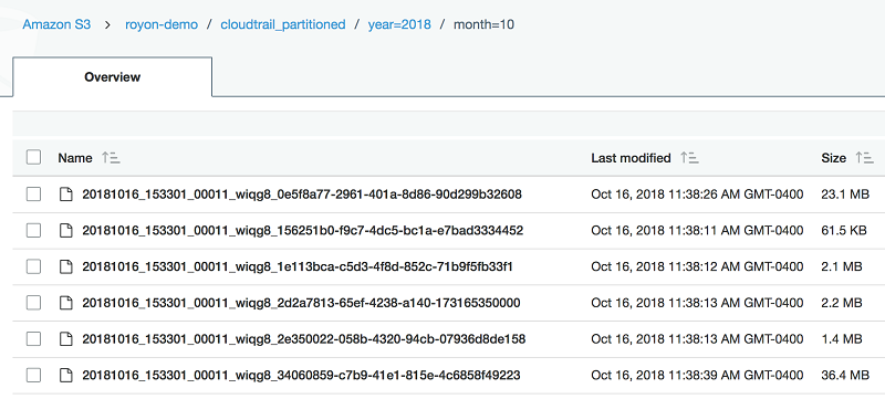
The third use case I want to highlight where CTAS can be of value is taking an existing unoptimized dataset, converting it to Apache ORC and partitioning it to better optimize for repeated queries. We’ll take the last 100 days of CloudTrail events and partition it by date.
Notice that I’ve added a WITH clause following the CREATE TABLE keywords but before the AS keyword. Within the WITH clause, we can define the table properties that we want. In this particular case, we declared “year” and “month” as our partitioning columns and defined ORC as the output format. The reason I used ORC is because CloudTrail data may contain empty columns that are not allowed by the Parquet specification, but are allowed by ORC. Additionally, I defined the external S3 location to store our table. If we don’t define an external location, Athena uses the default query result S3 location.
The resulting S3 destination bucket looks similar to the following example:
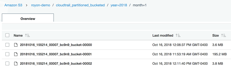
An additional optimization supported by Athena CTAS is bucketing. Partitioning is used to group similar types of data based on a specific column. Bucketing is commonly used to combine data within a partition into a number of equal groups, or files. Therefore, partitioning is best suited for low cardinality columns and bucketing is best suited for high cardinality columns. For more information, see Bucketing vs Partitioning.
Let’s take the previous CTAS example and add bucketing.
And this is what it looks like in S3:
Here is an example query on both a partitioned table and a partitioned and bucketed table. You can see that the speed is similar, but that the bucketed query scans less data.
Partitioned table:

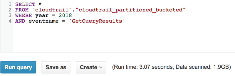
Partitioned and bucketed table:
Conclusion
In this post, we introduced CREATE TABLE AS SELECT (CTAS) in Amazon Athena. CTAS lets you create a new table from the result of a SELECT query. The new table can be stored in Parquet, ORC, Avro, JSON, and TEXTFILE formats. Additionally, the new table can be partitioned and bucketed for improved performance. We looked at how CTAS helps with three common use cases:
- Reducing a large dataset into a smaller, more efficient dataset.
- Selecting a subset of the columns and rows to only deliver what the consumer of the data really needs.
- Partitioning and bucketing a dataset that is not currently optimized to improve performance and reduce the cost.
Additional Reading
If you found this post useful, be sure to check out How Realtor.com Monitors Amazon Athena Usage with AWS CloudTrail and Amazon QuickSight.
About the Author
 Roy Hasson is a Global Business Development Manager for AWS Analytics. He works with customers around the globe to design solutions to meet their data processing, analytics and business intelligence needs. Roy is big Manchester United fan cheering his team on and hanging out with his family.