AWS Public Sector Blog
Building a Serverless Analytics Solution for Cleaner Cities
Many local administrations deal with air pollution through the collection and analysis of air quality data. With AWS, cities can now create a serverless analytics solution using AWS Glue and AWS QuickSight for processing and analyzing a high volume of sensor data. This allows you to start quickly without worrying about servers, virtual machines, or instances, so you can focus on your core business logic to help your organization meet its analytics objectives.
You can pick up data from on-premises databases or Amazon Simple Storage Service (Amazon S3) buckets, transform it, and then store it for analytics in your Amazon Redshift data warehouse or in another S3 bucket in a query-optimized format. In this blog, we will read PM2.5 sensor data, transform the dataset, and visualize the results.
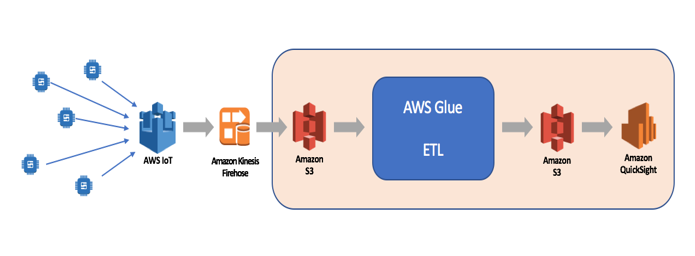
Figure 1: High level architecture of serverless analytics for air pollution analysis.
Data Collection
In a real-life scenario, you would start with data acquisition by leveraging services like AWS Greengrass, AWS IoT, or AWS Kinesis Firehose. In this example, our data will be stored in S3 buckets and we will be working with two data sources: raw sensor data in CSV files and sensor meta-data in JSON and CSV format.
AWS Glue, a set of services to do ETL – extract, transform, and load – is working with a data catalog containing databases and tables. The air pollution data is stored as JSON files in S3 buckets. Those files will be analyzed manually or automatically in a given context (database) and the data format(s) will be used to create schemata (tables). In the data catalog, you can also find the processes to inspect the data (crawlers) and data parsers (classifiers).
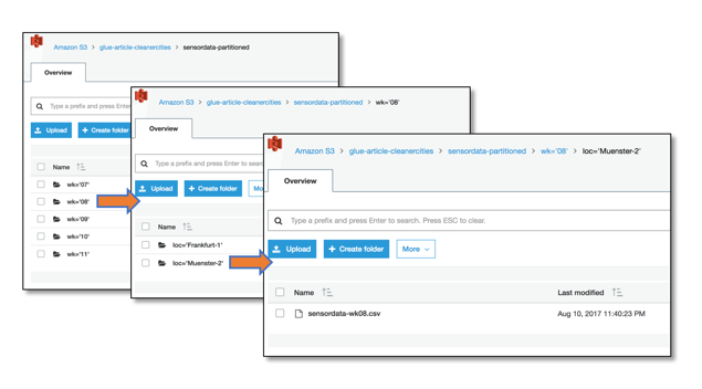
Figure 2: How data is organized in the S3 bucket
Creating a Crawler
By using the AWS Glue Crawler, defining schemata can be done automatically. Point the crawler to look for data and it will recognize the format based on built-in classifiers. You can write your own custom classifiers if needed. In cases where you cannot use the crawler, the data structure can also be defined manually.
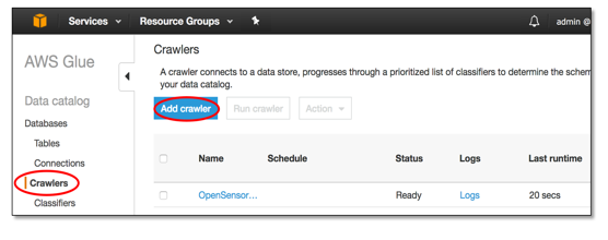
Figure 3: Adding a Glue Crawler
Switch to “crawlers” in the “data catalog” section. For automatically analyzing data structures, click “add crawler” and follow the wizard:
- Provide a name and an IAM role for the crawler. Check the documentation for the permissions a crawler needs in order to function. You can provide a description and custom classifiers in this stage if you need one.
- Enter one or more data sources. For S3 data, choose the bucket and, if necessary, the folder. By default, the crawler will analyze every subfolder from the starting point and you need to provide an exclude pattern if this is not desired.
- Define a schedule for when to execute the crawler. This is useful if the source data is expected to change. Since our data won’t change structurally, we’ll choose “run on demand.”
- Choose the output of a crawler – the database. Use an existing one or let the crawler create one. Remember that the crawler will inspect the files in the S3 bucket and every distinct data structure identified will show up as a table in this database.
- Review and confirm.
Adding a Custom Classifier
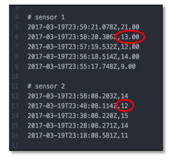
Figure 4: Showing subtle difference in input data formats
We could launch the crawler now, but our sensors provide values in floating point and in integer format. The crawler would recognize them as different tables. You can see how this works by default and then delete the tables afterwards. Or, to import the files as one data structure, we can introduce our own data classifier for CSV-based data.
On the “data catalog” tab, choose section “classifiers” and add a new classifier by defining a Grok pattern and additional custom patterns if needed. In our example, data is structured as CSV with two columns. The first column is a timestamp; the second is a number. All analyzed files that match this pattern will end up in the same table.
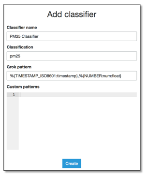
Figure 5: Adding a classifier
Working with Partitions
We had hierarchical structure in our data. There were folders for the week number of the data and there were folders for the sensor location. Glue is able to use this information for the datasets. While our data files contain two components (timestamp and value), the crawler created a schema containing four columns.
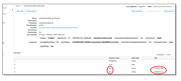
Figure 6: Glue working with partitions
Glue automatically added the information contained in the structure of our data store as fields in our dataset. The names of the columns are also taken from the folder names given in our data store. Instead of just having a folder named “Frankfurt”, we had one called “loc=’Frankfurt,’” which is interpreted as column name and value. If you are not able to follow that naming scheme, the additional fields will be introduced as well, but they will have generic names, which can be renamed in the transformation part of our Glue-based ETL.
Defining a database and table manually
The destination for our data is S3, but in JSON files. We can’t use a crawler to automatically define this because our destination files do not exist yet. Go to the “data catalog” section, select “databases,” and select “add database.” You need to provide a name – details will follow in the tables. To define them, select your database, click on “Tables in <your-database-name>” and start the table wizard by clicking “add tables.” Following the wizard, you can provide the data location, its format, and manually define the data schema. In our example, we will only have a simple transformation and Glue will be able to create the destination table.
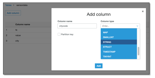
Figure 7: Glue, table wizard.
Moving and transforming data
In AWS Glue, a Job will handle moving and transforming data. A Glue Job is based on a script written in a PySpark dialect, which allows us to execute certain built-in and custom-defined transformations while moving the data. We can strip decimal digits from our PM2.5 values and we will add a city code to our records.
Select “jobs” in the ETL section and start the wizard for adding a new Job. We will keep our example simple and let Glue generate a script.
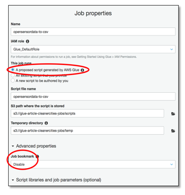
Figure 8: Authoring a job in Glue
Select data source(s) and data target. You can filter the list of tables to find the one that our crawler created. For the target, you can search for an existing one or create one now. In the case of S3 buckets, make sure that they really exist – otherwise, your script might fail.
We disabled “job bookmark.” Glue knows what data has been processed by maintaining a bookmark. If you are testing or debugging a script, it’s a good idea to have this disabled; otherwise, nothing will happen after you have processed your data once.
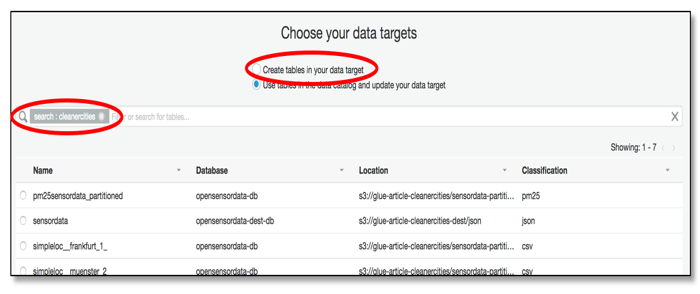
Figure 9: Choosing targets
Now that Glue knows the source and target, it will offer us a mapping between them. You can add columns and change data types.
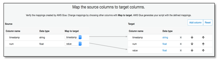
Figure 10: Mapping source to target in Glue
In the background, Glue will generate the script as needed. You will be able to change it from here. Insert pre-defined transformation templates and adapt them to your data structures.
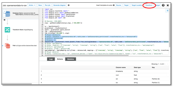
Figure 11: Editing your ETL job in Glue
Launching simple ETL scripts will take our data into our destination bucket in the format and with the column names we defined. It’s possible to have more than one destination. You can decide to write your data to JSON files and CSV files within one ETL job.
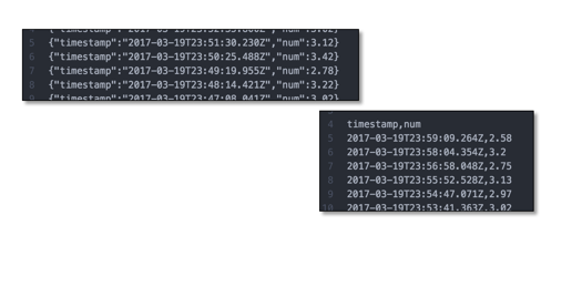
Figure 12: Glue transformations in action
In a second transformation, we join the sensor measurement data with the sensor meta data to add a location code to the name of the city. Therefore, we need to access a second data source and join both sources during the ETL job. You can find the complete job script at s3://glue-article-cleanercities/resources/.
For this, please create and run a new crawler for the file s3://glue-article-cleanercities/sensordata-metadata/sensor_location.csv. Edit the resulting table schema to provide some meaningful column names like “city” and “code” instead of “col0” and “col1.”
Now, edit the job script to include this new data source. Select the “source” button and enter the respective values in the inserted code snippet. Then join both tables on the fields “loc” and “city.” Place the cursor after the “ApplyMapping” snippet, push “Transform” and select “Join.”
## @type: Join
## @args: [keys1 = [“loc”], keys2 = [“city”]]
## @return: join1
## @inputs: [frame1 = applymapping1, frame2 = datasource1]
join1 = Join.apply(frame1 = applymapping1, frame2 = datasource1, keys1 = [“loc”], keys2 = [“city”])
And that’s it. Starting the job again will result in records that contain values of both data sources.
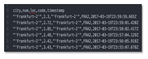
Figure 13: Results from both sources
Analyzing Data in S3 Buckets
There are many options to process and analyze data on AWS, such as AWS Redshift or AWS Athena. For a quick visual analysis of our data, let’s use AWS Quicksight. Quicksight is able to consume data from S3 buckets and allows you to create diagrams in a few clicks. You can share your analysis with your team and they can be applied to new data quickly and easily.

Importing and visualizing sensor data with a serverless architecture can be a first step to improve air quality for citizens. Taking the next steps, such as correlating air quality with factors like weather or time of day, training artificial intelligence systems and influencing traffic flows based on machine learning predictions, can be achieved by leveraging AWS services without having to manage a single server.
Whether it is air pollution monitoring and analysis, threat detection, emergency response, continuous regulatory compliance, or any other public sector big data and analytics use case, AWS services can help you build a complex analytics workload quickly, easily, and cost effectively.
A post by Ralph Winzinger, Solutions Architect at AWS, and Pratim Das, Specialist Solutions Architect– Analytics at AWS.